Appendix 4

Data Acquisition and Analysis

To prepare to measure and analyze data the following steps are recommended.

Install nanoVNA hardware and nanoVNA-qt software

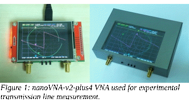
While many VNAs are suitable for these experiments, the NanoVNAV2 family of nanoVNAs are a particularly good value which make high quality measurement affordable. Most of these experiments have used the nanoVNA-v2-Plus4 which can be operated from LF to well into the microwave region while having continuous self-calibration as pictured in Figure 1.

Information and links about this VNA are available at

https://groups.io/g/NanoVNAV2

which provides information about where to obtain one. In addition, it has links to

NanoVNA-QT software

which is used to interface to the VNA from a computer by way of a USB cable.

It is not required to use this particular VNA. Any modern VNA that is capable of performing a 1-path 2-port measurement and saving the results as a Touchstone .s2p file will suffice.

VNA Connection, Test Cables and Calibration

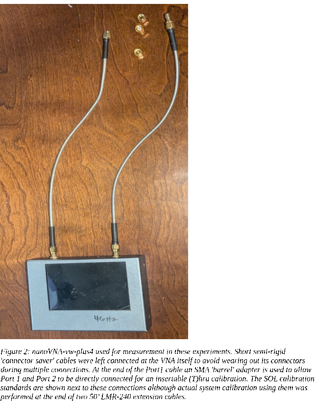
Because the lines being measured can be as much as 100 feet long, the test ports of the VNA need to be extended with test cables to reach and connect to whichever test fixture is in use. For the experiments shown, two approximately 50 foot lengths of LMR-240 cable fitted with male SMA connectors were used. In addition, two short semi-rigid .141” cables were used at the VNA as “connector savers” so that repeated connections at the VNA would only wear out or harm a cable and not the VNA SMA connectors. To connect at both ends of the 50 cables, SMA-SMA adapters are used.

A convention creating a female SMA connection on Port 1 and a male connection from VNA Port 2 was used, both the VNA location and at the ends of the long test cables. By using different gender connection types, the ‘thru’ calibration of the VNA is always insertable. That is, no additional calibration devices are required beyond the SOL devices used. The “(T)hru was simply a direct connection.

For these measurements quality 50 ohm calibration standards were available. Generally even the NanoVNA models are supplied with adequate (S)hort, (O)pen and (L)oad standards as shown in Figure 2. These give good results for LF – VHF measurements.

The 50’ test cables are insertable extensions of the connector saver connections at the VNA. SMA-SMA female adapters are used to accomplish this. In operation SMA connections are torqued to at least 9 inch-pounds and monitored to be sure they don’t loosen during use.

Install Python and a virtual environment

Creating a virtual environment for Python is a way to isolate your project’s dependencies so that different projects don’t conflict with each other. Here’s how to do it, step by step:

Prerequisites

Make sure you have Python 3.6 or newer installed.

You can check this with:

python3 --version

or on Windows:

python --version

If you don’t have Python, download it from python.org/downloads.

Step-by-Step: Create and Use a Virtual Environment

1. Navigate to your project folder

Open a terminal or command prompt and go to the directory where you want your project:

cd ~/my_project

2. Create the virtual environment

Run:

python3 -m venv venv

or on Windows:

python -m venv venv

This creates a new folder called venv that contains the isolated Python environment.

(You can replace venv with any name you prefer, e.g. .venv or env.)

3. Activate the virtual environment

• On macOS / Linux:

  source venv/bin/activate

• On Windows (PowerShell):

  .\venv\Scripts\Activate.ps1

• On Windows (Command Prompt):

  venv\Scripts\activate

When activated, your terminal prompt will change to show the environment name, for example:

(venv) $

4. Install packages inside the environment

Once activated, you can install packages as usual, but they’ll be isolated to the virtual environment:

pip install numpy matplotlib scikit-rf

5. Verify it’s working

You can check installed packages:

pip list

Or confirm Python is using your virtual environment:

which python

(on macOS/Linux)

or

where python

(on Windows)

6. Deactivate when done

To exit the virtual environment:

deactivate

Jupyter Notebook

With Python installed and operating within a virtual environment Jupyter notebook is a very useful context to analyze and render collected data. It offers an easy way to encapsulate, share and collaborate on experiments. It is freely available here

Jupyter Notebook

Experiment X is available for download which will immediately provide tools, present as “cells” within a notebook, which provide an easy starting point for replicating and expanding on transmission line experiments.

From this point on, precede any work by entering the virtual environment first. This will provide an environmental “sandbox” to isolate the project from any other installations that might exist on the computer.

Once the terminal command line shows the (venv) prefix indicating that the environment is active, start Jupyter Notebook.

If all work are done in this context you will have an isolated environment to examine a previously created project located in its own subdirectory as well as to create and perform your own experiments.

All of these may be shared and collaborated on with others.