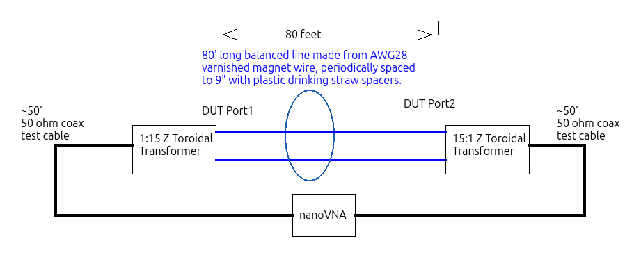
Figure 1: The block diagram of this experiment shows the flux-coupled toroidal transformers at the ends of the 80' long balanced line under test.
This experiment is a measurement of an 80 foot length of 2-conductors of AWG #28 magnet wire separated by 9” drinking straw spacers as depicted in Figure 1. Some extra detail of this simple measurement is provided in order to describe the environment and analyses common among many of the following experiments.
Figure 1:
The block diagram of this experiment shows the flux-coupled toroidal
transformers at the ends of the 80' long balanced line under test.
At this spacing the conventional formulae for balanced line impedance predict that this should be
The test fixture turns ratio would suggest that it could be appropriate to match 50 ohms to a load impedance of
which while not precise would be an approximate match were the line impedance as high as the prediction.
This line was previously fabricated several years ago but not carefully measured at that time. This measurement is fixtured using 5:19 turn, lumped flux-coupled transformers at each end. These are described in Appendix 1. For this experiment the VNA was SOLT calibrated in a reference impedance of 754 ohms located at the plane of the line connections.
The band-limited nature of the impedance transformer indicated that a measurement in 1 MHz steps over a 1MHz to 100 MHz frequency span might be appropriate.
The experimental environment was above a wooden fence having 8 foot post spacing and horizontal wooden planks. It also had metal rabbit wire mesh stretched along its length and from the top plank to the earth. The LUT was kept well above this fencing after determining that any further increase in the height had no measurable effect on any of the results.
Illustration 1 is a photograph of that environment which is similar for all of the experiments.
Illustration 2 provides a close-up view of the Port 1 end of the system with short clip lead connections to allow switching between measurement of calibration standards and of the LU
NanoVNA-qt1 running on a Windows OS laptop was connected to NanoVNA V2 Plus4 VNA and used to perform a SOLT calibration using a leaded 754 ohm resistor ‘load’, alligator clip lead connections for the ‘short’ as well as ‘thru’ calibration standards, 1-path 2-port S11 and S21 measurements of the 80 foot long LUT were thereby performed.
Both the calibration and data measurements were made using NanoVNA-qt software which saved the measured, error-corrected data into a Touchstone format .s2p file. To save it, the measurement was repeated and saved into S12 and S22 fields as well in order to provide all four S-parameters within the file for later analysis. The nearly identical additional parameters were not actually used as part of rendering the data.
Much of the analysis for this experiment as well as the ones which follow was done within Jupyter Notebook2. This is a convenient environment that can natively execute and render the output of Python code. The Python user code used for analysis is only a small program but uses the scikit-rf and matplotlib Python packages These are rich libraries which handle most of the complexities and make data presentation and time domain analysis easy to access with only a few lines of user code needed.
An entire directory containing the notebook file and also data and image files is available so that a user interested in replicating this experiment or creating additional ones has a convenient starting point.
Time domain gating3 of both the reflection and transmission measurements allows removing unwanted reflections from the measurement and analysis and display of only the first reflection and first transmission components. The rendered data in Figure 4 shows both raw .s2p as well as time gated results.
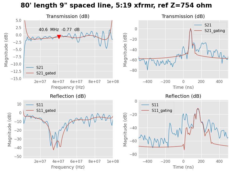
Figure 2:
Frequency, time and time gated measurement plots for
X-3p8-9-28-80-L-754.
This result was expected from the band limited nature of the toroidal transformers and from the difficulty in maintaining constant environments between calibration and measurement phases of the VNA operation. Later experiments have included another toroidal core to improve balance of the fixtures and remove common mode current on the test port cables.
Even with these measurement imperfections, quite low attenuation for this length of line is reported. This low transmission attenuation exceeds the specifications for even the reasonably high performance LMR240 coaxial test cables being used as part of the overall test fixture. Manufacturer’s specification for this cable would indicate a corresponding loss at 40 MHz of around 1.2 dB for the same physical length.
This low attenuation agrees with handbook estimates for balanced transmission lines of higher impedance. Even though the conductor diameters are considerably smaller for the balanced line than for the coaxial center conductors of the LMR240, because the impedance is higher and currents correspondingly lower, conductor losses are much less. This is an inherent advantage of higher impedance lines using conductors made from real materials.
1NanoVNA-QT https://nanorfe.com/NanoVNA-v2-software.html
2Jupyter Notebook https://jupyter.org/
3APPLICATION NOTE Time Domain Analysis Using a Network Analyzer , Keysight